Non Linear Least Squares Localization

Non Linear Least Squares

Our model consist of i anchors and 1 beacon
\( x \) is the unknown beacon position
\( u \) is the known positions of each ith anchor
\( y \) is the given measurement of the distance between each ith anchor to the beacon

Model,

\[ \begin{align} y_i \approx \sqrt{(x_0 - u_{i0})^2 + (x_1 - u_{i1})^2} \end{align} \]

ith Residual,

\[ \begin{align} f_i(x) = \sqrt{(x_0 - u_{i0})^2 + (x_1 - u_{i1})^2} - y_i, \quad i=0,1,2 \end{align} \]

Jacobian,

\[ \begin{split}\begin{align} &J_{i0} = \frac{\partial f_i}{\partial x_0} = \frac{x_0 - u_{i0}}{ \sqrt{(x_0 - u_{i0})^2 + (x_1 - u_{i1})^2} } \\ &J_{i1} = \frac{\partial f_i}{\partial x_1} = \frac{x_1 - u_{i1}}{ \sqrt{(x_0 - u_{i0})^2 + (x_1 - u_{i1})^2} } \end{align}\end{split} \]

Python code,

import numpy as np
from scipy.optimize import least_squares
import matplotlib.pyplot as plt
import matplotlib.patches as patches

def model(x, u):
    return ((x[0] - u[:,0])**2 + (x[1] - u[:,1])**2)**0.5

def residual(x, u, y):
    return model(x, u) - y

def jacobian(x, u, y):
    J = np.empty((u.shape[0], x.size))
    den = ((x[0] - u[:,0])**2 + (x[1] - u[:,1])**2)**0.5
    J[:,0] = (x[0] - u[:,0]) / den
    J[:,1] = (x[1] - u[:,1]) / den
    return np.nan_to_num(J)

Weighted Non Linear Least Squares

Model

\begin{align} y_i \approx \sqrt{(x_0 - u_{i0})^2 + (x_1 - u_{i1})^2} \end{align}

Weight,

\begin{align} w_i = {\sigma}^2y_i \end{align}

ith Residual,

\begin{align} f_i(x) = w_i\sqrt{(x_0 - u_{i0})^2 + (x_1 - u_{i1})^2} - w_iy_i, \quad i=0,1,2 \end{align}

Jacobian,

\begin{split}\begin{align} &J_{i0} = \frac{\partial f_i}{\partial x_0} = \frac{w_i(x_0 - u_{i0})}{ \sqrt{(x_0 - u_{i0})^2 + (x_1 - u_{i1})^2} } \\ &J_{i1} = \frac{\partial f_i}{\partial x_1} = \frac{w_i(x_1 - u_{i1})}{ \sqrt{(x_0 - u_{i0})^2 + (x_1 - u_{i1})^2} } \end{align}\end{split}

Python code,

def model_w(x, u):
    return ((x[0] - u[:,0])**2 + (x[1] - u[:,1])**2)**0.5

def weight(y):
    return 1 / y**2

def residual_w(x, u, y):
    w = weight(y)
    return w * model(x, u) - w * y

def jacobian_w(x, u, y):
    w = weight(y)
    J = np.empty((u.shape[0], x.size))
    den = ((x[0] - u[:,0])**2 + (x[1] - u[:,1])**2)**0.5
    J[:,0] = w * (x[0] - u[:,0]) / den
    J[:,1] = w * (x[1] - u[:,1]) / den
    return np.nan_to_num(J)

This is a more advanced way of selecting weights (see choosing-weights)

\begin{align} p_i = \frac{n}{\sigma_g^2 + d^2\sigma_m^2} \end{align}

where,

n is the number of observations
d is the distance
\( \sigma_m \) is the standard deviation of the measuring device
\( \sigma_g \) is the standard deviation of the measuring device and of centering the device

Test Data

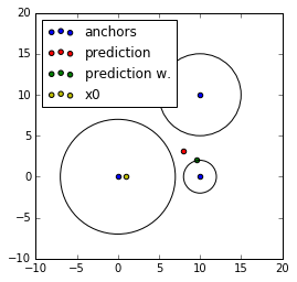
u = np.array([[0,0],[10,0],[10,10]])
y = np.array([7, 2, 5])
x0 = np.array([1,0])

result   = least_squares(residual, x0, jac=jacobian, bounds=([-10,10]), args=(u, y), verbose=1)
result_w = least_squares(residual_w, x0, jac=jacobian_w, bounds=([-10,10]), args=(u, y), verbose=1)

%matplotlib inline
plt.scatter(u[:,0], u[:,1], label='anchors')
plt.scatter(result.x[0], result.x[1], label='prediction', c='r')
plt.scatter(result_w.x[0], result_w.x[1], label='prediction w.', c='g')
plt.scatter(x0[0], x0[1], label='x0', c='y')
for i in range(u.shape[0]):
    plt.gca().add_patch(
        plt.Circle(tuple(u[i]), y[i], fc='none')
    )
plt.axis('scaled')
plt.legend(loc="upper left")
plt.show()

png